NOMAD | BL-1B | SNS

Introduction

The NOMAD auto-reduction routine is a wrapper around the TotalScatteringReduction module which is the backbone of the MantidTotalScattering package for neutron total scattering data reduction. In the TotalScatteringReduction method, different scheme can be specified for grouping detectors at both the data processing and output stage. There are two commonly used ways of grouping detectors – group detectors by physical banks and group all detectors into a single bank. For NOMAD auto-reduction, both of the approaches are implemented. The multi-banks mode is advantageous in terms of using as much of the high-angle bank (which is with high resolution) as possible. Here, the resolution of the total scattering pattern in \(d\)-space can be derived as follows,

\[2d\,sin\theta = \lambda \Rightarrow \Delta d = \frac{\lambda}{2}\frac{cos\theta}{sin^2\theta} \Rightarrow \frac{\Delta d}{d} = cot\theta\tag{1} \]

from which one can see that the resolution is increasing monotonically as the increase of the scattering angle. One of the biggest advantages of the single-bank mode is that it can directly give a single \(Q\)-space total scattering pattern for which the Fourier transform can be performed automatically, given necessary input parameters pre-configured.

Upon the reduction of each individual run at the auto-reduction stage, the align and focused data will be saved to a certain location (which is specific to each experiment) as cache files. Meanwhile, the individual reduction configuration will be saved as JSON file. Afterwards, the auto-reduction engine will check the output directory for existing JSON files and search (by sample title) for all runs that are similar to the current run. Here, by similar runs, we mean all those repeated runs for the same sample under the same measurement condition. Then a merged JSON file will be generated to incorporate all those similar runs, after which a TotalScatteringReduction run will be executed with the merged JSON file as the input. Once again, both the single-bank and multi-banks mode will be used for running the merged JSON input. After all, all those merged JSON input will be finally merged into a comprehensive JSON file, which then can be later imported into ADDIE for manual reduction purpose. In fact, given the current iterative approach (as detailed below) of running the auto-reduction routine, in most cases, manual reduction is not necessary. However, in case some improper configuration at the auto-reduction stage, one can perform the manual reduction using ADDIE (as detailed here) via interfacing with the generated JSON file.

Given the proper background subtraction and instrument effect normalization and the necessary corrections (absorption effect, multiple scattering effect, etc.) being in place, one is expecting the reduced total scattering will be sitting on an absolute scale, i.e., the data is directly comparable with a theoretical calculation of the total scattering pattern upon a structure model consistent with the measured sample, without the need for an extra scale factor. In such a situation, the reduced \(S(Q)\) data [as defined below in Eqn. (2)] should asymptotically approach the self-scattering level [see Eqn. (3) below] in the high-\(Q\) region.

\[S(Q) = \frac{1}{N}\sum_{j,k}b_jb_k\frac{sin(Qr_{jk})}{Qr_{jk}}\tag{2}\]

\[\langle b^2\rangle = \sum_ic_ib_i^2\tag{3}\]

where \(c_j\), \(c_k\) refers to the number concentration of atom species \(j\) and \(k\), respectively. \(b_j\) and \(b_k\) is for the scattering length of each species, and \(N\) is the total number of atoms in the material. However, in practice, it is almost always the case that even the mass density is measured correctly and all the necessary corrections are in place, the high-\(Q\) level will be slightly off the self-scattering level. With this regard, the packing fraction tweaking factor is introduced for adjusting the high-\(Q\) level towards the self-scattering level – equivalently, one can also imagine this as tweaking the effective density of the material. At this point, one may wonder why we do not directly scale the data to the self-scattering level by simply multiplying a scale factor, since anyhow tweaking the packing fraction seems to be doing exactly the same thing. However, this is not true, since tweaking the packing fraction will not only induce a scale factor but also will induce a non-uniform impact on the absorption correction across the \(Q\)-space. This is also the reason why one has to re-do the absorption correction any time the packing fraction is tweaked. So, the implementation here is that after each auto-reduction run, we will be checking the high-\(Q\) level of the output \(S(Q)\) pattern, compare it to the self-scattering level and suggest a new packing fraction. Such a procedure will continue until the packing fraction value is converged. Usually, we found that the packing fraction value will converge after 2 or 3 cycles.

N.B. The absorption calculation (no matter which approach is used, such as numerical integration or Monte Carlo ray tracing) is computationally heavy. The major reason is that the absorption strength is dependent on the flying path and therefore each single detector physically located at different location will give different absorption spectra as the function of wavelength. In principle, all detectors should be treated explicitly which will accumulate the processing time and in practice, the large amount of detectors (for example, on NOMAD, there are more than 100, 000 detectors) will make the computation heavy for the absorption correction. Therefore, if staying with the pixel-by-pixel level of correction for the absorption effect, the iterative manner of reducing the total scattering data, as detailed above, will make the auto-reduction running time unrealistically long. Concerning this, we implement a routine for performing the absorption calcualtion in a group manner – see here for relevant discussion about the performance boost in the case of absorption correction.

In summary, the NOMAD auto-reduction routine can,

1. process individual runs and sum all similar runs automatically.

2. cache all processed runs properly for later manual reduction to load for saving processing time.

3. iterate until the packing fraction tweak factor is converged, trying to bring the data as close to an absolute scale as possible.

4. reduce the data in both single-bank and multi-banks mode – the former one will be automatically Fourier transformed to obtain the pair distribution function.

5. detect calibration and all the characterization runs (such as vanadium, empty container and empty instrument runs) so that the data reduction step will be skipped. Specifically for the calibration run, if the corresponding calibration file was not ever generated, the calibration routine will be called automatically to prepare the calibration file from the calibration run.

6. be easily configurable, by concentrating all tweaking parameters in dedicated files in either json or CSV format – details about how to configure the inputs for the auto-reduction will be covered below.

7. save input configuration for both the indiviudal and sum runs for later checking and re-use purpose – as the auto-reduction is running during the experiment, all those input configuration for sum runs will be accumulated and saved as a compact JSON file at an IPTS specific location (see the section Location of Files down below for detailed information) so that later manual reduction with ADDIE (see details here) can direcly load it into the table for configuring manual data reduction.

Implementation Flowchart

Here, the flowchart of the NOMAD auto-reduction is presented. As mentioned above, the auto-reduction routine is just a wrapper around the TotalScatteringReduction module, the details of which can be found in the MTS workflow section.

N.B. In the diagram, the red node is either representing a module, the starting point, or the ending point of the flow. The green node is for input parameters of a certain routine. The blue node with the same label text is representing the same parameter that is needed at different spots.

Prepare auto-reduction

There are several steps to go through on the user side (in practice, it is usually the instrument scientist who is local contacting the experiment) to configure the auto-reduction before the experiment starts. This will be covered here and it will be presented in the order of need-to-do frequency, i.e., the top one is always needed, the next one is less frequent, and so on.

1. Prepare the sample information.

   After users check in their samples, the information about the samples will be available in the ORNL ITEMS database, and each sample is with a unique sample ID. The same set of sample ID will be used for the experiment. This means before the experiment starts, one can fethc the sample information from the database and populate them into a file that can be found by the auto-reduction routine. Meanwhile, since the absorption correction only depends on the sample information and the instrument geometry, the absorption coefficient as the function of wavelength can be pre-calculated once the sample information is collected. Again, the calculated absorption coefficient can be cached into files that can be found by the auto-reduction routine.

   With this regard, a utility called abs_pre_calc was developed to perform the series of actions in a semi-auto manne, as detailed below,

   1.1. Connect to the analysis cluster using either browser or Thinlinc.

   1.2. Launch a terminal, by going to Applications \(\rightarrow\) Terminal, as shown here,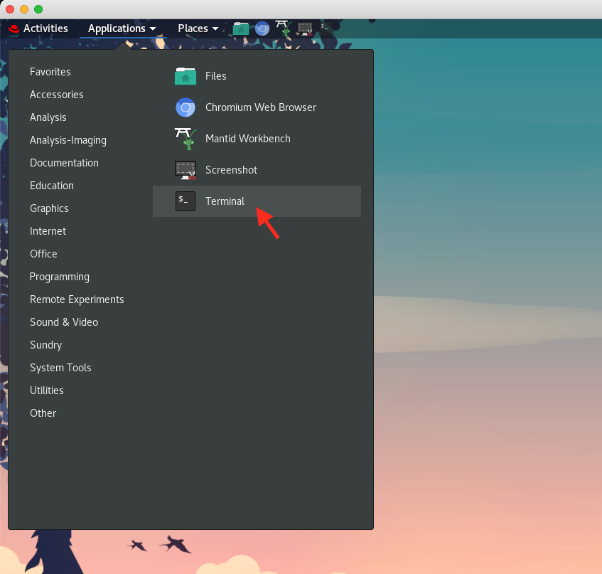

   

   1.3. Execute abs_pre_calc 12345 where 12345 is a representative IPTS number.

   N.B. Execute abs_pre_calc followed by nothing will show the usage of the utility. Execute abs_pre_calc -h will show the detailed documentation of the utility.

   1.4. Here, we take the IPTS-28922 (which contains the instrument calibration and characterization runs) as an example. After we execute abs_pre_calc 28922 from the terminal, the sample information will be fetched from the ITEMS database and the information will be saved into a CSV file (located at an IPTS specific location, analogous to /SNS/NOM/shared/mts_abs_ms/IPTS-28922 for current example), after which the spreadsheet application (LibreOffice on analysis) will be launched to open the saved sample information CSV file. This is the spot where one can correct the sample information – usually when general users check in their samples, the information may not be entered properly so some manual efforts are needed here for correcting those information. The necessary information is as listed here,

   • Chemical Formula – the follow formats are accepted, Sr Ti O3, Sr1 Ti O3, (Sr)1.0 Ti O3, Sr (Ti) (O16)3, where the bracket is useful to specify the isotope.

   • Mass Density – we suggest to use the actually measured mass density. However, one can also use the theoretical mass density here, since anyhow the effective density will change according to the packing fraction tweaking factor.

   • Packing Fraction – one can start with an not-too-far-off arbitrary value, e.g., 0.8, since the auto-reduction engine will iteratively adjust its value on-the-fly.

   • Container Type – The type of the container being used for holding the sample. On NOMAD, usually, the 3 mm capillary and 6 mm PAC can are commonly used, and we can input C or P as a short name for each. Sometimes, if users have ever put in the information for containers to be used when checking in their samples, the container type information will be fetched from the ITEMS database at current stage. In that case, one may only need to check the automatically fetched container type is valid. The acceptable container type is,

     • Quartz03

     • QuartzTube03

     • PAC03

     • PAC06

     • PAC08

     • PAC10

     • P

     • C

     • O

     We have mentioned that P and C are used as the shortname to represent the Quartz03 and PAC06 container, respectively. As for O type, we use this shortname to represent any other type of containers.

     If any standard container type is specified (i.e., all the acceptable values listed above except O), the following two entries Shape and Radius DO NOT need to be provided – the shape and radius for each standard type of container can be found in the table below. Otherwise, the shape and radius information for the container being used should be provided as instructed below.

     Container	Inner Radius (cm)	Shape
     QuartzTube03	0.14	Cylinder
     PAC03	0.135	Cylinder
     PAC06	0.295	Cylinder
     PAC08	0.385	Cylinder
     PAC10	0.46	Cylinder

   • Shape – usually it is Cylinder for commonly used sample container (e.g., the PAC CAN or silica capillary used on NOMAD). However, in some cases, other types of container may be used and more available shape can be found in the Mantid documentation about Geometry and ContainerGeometry.

   • Radius – this specifies the inner radius of the container being used (for non-cylindrical and non-spherical containers, this is not relevant).

   N.B. Up-to-date information about containers geometry can be found in the Mantid source code here.

   • Height – sample height in container

   • Abs Method – specify the method to be used for performing the absorption pre-calculation. Here, short names of the absorption correction method will be used in the CSV file for saving the user input effort. Here follows is presented a table containing the correspondence between the short name and the method,

     Short Name	Absorption Correction Method
     None	No absorption correction
     SO	SampleOnly
     SC	SampleAndContainer
     FPP	FullPaalmanPings

   Details about theoretical background for each type of absorption correction method can be found here.

   • MS Method – specify the method to be used for multiple scattering correction. The absorption and multiple scattering calculation is implemented in the same code base and more details can be found here. Below is presented a table containing the correspondence between the short name and the method,

     Short Name	Multiple Scattering Correction Method
     None	No multiple scattering correction
     SO	SampleOnly
     SC	SampleAndContainer

   Once the table is configured properly, one can proceed to close the spreadsheet application so the utility will continue to the next action, which is mainly about the absorption and multiple scattering calculation, if specified to be performed. There are several aspects worth to mention,

   • Once the spreadsheet application is closed, the utility will be checking the validity of those necessary entries as detailed above in the CSV file and if invalid entries are spotted, the CSV file will be automatically opened again for users to correct those information or fill in those missing ones. The invalid entries will be printed to the terminal console so that users can get an idea about what is going wrong.

   • If an existing sample information file is found, the utility will check the entries in the existing file and compare with the ITEMS database to populate those additional samples as compared to last time running of the utility.

   • The pre-calculated absorption coefficient will be saved to IPTS specific directory with unique names corresponding to all parameters that determine the absorption coefficient. Taking the IPTS-28922 example as used above, the cached absorption calculation can be found at /SNS/NOM/shared/mts_abs_ms/IPTS-28922 on analysis. When the utility is running, it will check the IPTS specific directory to see whether the specified absorption calculation already exists. It will only proceed to the absorption calculation if not preceeding absorption calculation was found. Users, including the instrument team, will rarely need to check the cached absorption calculations.

   • The multiple scattering calculation, if specified to be performed, will be conducted altogether with the absorption calculation and they will be saved altogether as the effective absorption coefficient. Therefore, in terms of implementation and data flow internally in the calculation routine, adding in the multiple scattering correction is making no difference as compared to the case of absorption correction only. Details about such an implementation can be found here.

   The steps so far are summarized in the recorded GIF as below,

   

2. Prepare the characterization file.

   For reducing the measured data for users’ samples, a series of characterization runs need to be collected, including the calibration run, the vanadium run, the empty container run and the empty instrument run. Infomation about those characterization runs associated with the measurement for users’ samples should be pre-configured, usually by the instrument team. The characterization file is for such a purpose and on NOMAD, it can be found at. /SNS/NOM/shared/autoreduce/auto_exp.csv. The file format is follows,

   Run Start	Run End	Sample Env	Calib	Van	PAC	CAP	Other Can	MT
   181275	181278	Shifter	183057	179270	181279-181282	-	-	179271
   172400	-	Shifter	172394	172401	172397-172400	-	-	172402

   where each row is specifying a range of runs for which the characterization runs apply. If the Run End is - or empty, its value will be taken from the Run Start entry in the row just above. For those entries of the characterization runs, a single run or a series of runs are both acceptable. When specifying a series of runs, one can use the format like 181279-181282, or 181279, 181281-181282, or 181279, 181282.

3. Configure the parameters ONLY WHEN NEEDED.

   There are multiple parameters for controlling the behavior of the auto-reduction and they can be configured in a JSON file located at /SNS/NOM/shared/autoreduce/auto_config.json on NOMAD. In most cases, most of the parameters DO NOT need to be touched. However, there are several parameters that may need to be tweaked, as detailed here,

   Param Name	Function
   TMIN	Minimum time-of-flight (in \(\mu s\)) to truncate the data in TOF-space
   TMAX	Maximum time-of-flight (in \(\mu s\)) to truncate the data in TOF-space
   QMin	Lower limit of the \(Q\)-range used for the Fourier transform
   QMax	Upper limit of the \(Q\)-range used for the Fourier transform
   RMax	The upper limit of the generated pair distribution function
   RStep	The step of the generated pair distribution function

   There is a parameter OverrideUserConfig which controls whether the parameters listed in the table above from the central configuration file (i.e., /SNS/NOM/shared/autoreduce/auto_config.json) will override those from the user configuration. Starting from scratch, when the auto-reduction is running, it will copy over those parameters in the table to user configuration file in JSON format located at an IPTS specific location – taking the IPTS-28922 example, the user configuration file will be saved at /SNS/NOM/IPTS-28922/shared/autoreduce/auto_params.json. The next time when running the auto-reduction, if OverrideUserConfig is specified to be False, the existing user configuration file will be loaded and those loaded parameters will be used. Otherwise, the parameters from the central configuration file will be used and the user configuration file will be overwritten. Before the overwriting, the user configuration file will be backed up to the same directory as the existing file to keep the history. The backup file will be named as something like auto_params_backup_05262023_2.json, where 05262023 is the time stamp and 2 is a representative integer which is determined as the smallest number that guarantees a non-existing backup file. Here, the hash value for the backup file contents will be checked to guarantee that only unique parameters set will be backed up.

   N.B. The verison of the Mantid framework and the underlying MantidTotalScattering engine will also be populated into the user configuration file.

Once the preparation work is done properly, the autoreduction will be running smoothly in the background as the data are being collected and populated to analysis hard drive. The location of the reduced data will be introduced later.

Manual submission

In most cases, if the preparation work as detailed above has been done properly, the auto-reduction will be executed automatically, without us even realizing the existence of the reduction routine. However, in some cases, there may be the need to re-submit the autoreduction job, for example, when the initial inputs were found to be not suitable. This part then covers how to re-submit the auto-reduction job using the monitor web interface.

1. Go to NOMAD monitor, https://monitor.sns.gov/report/nom/.

2. There you will a list of IPTS’s – select the one you are interested in and have access to.

   

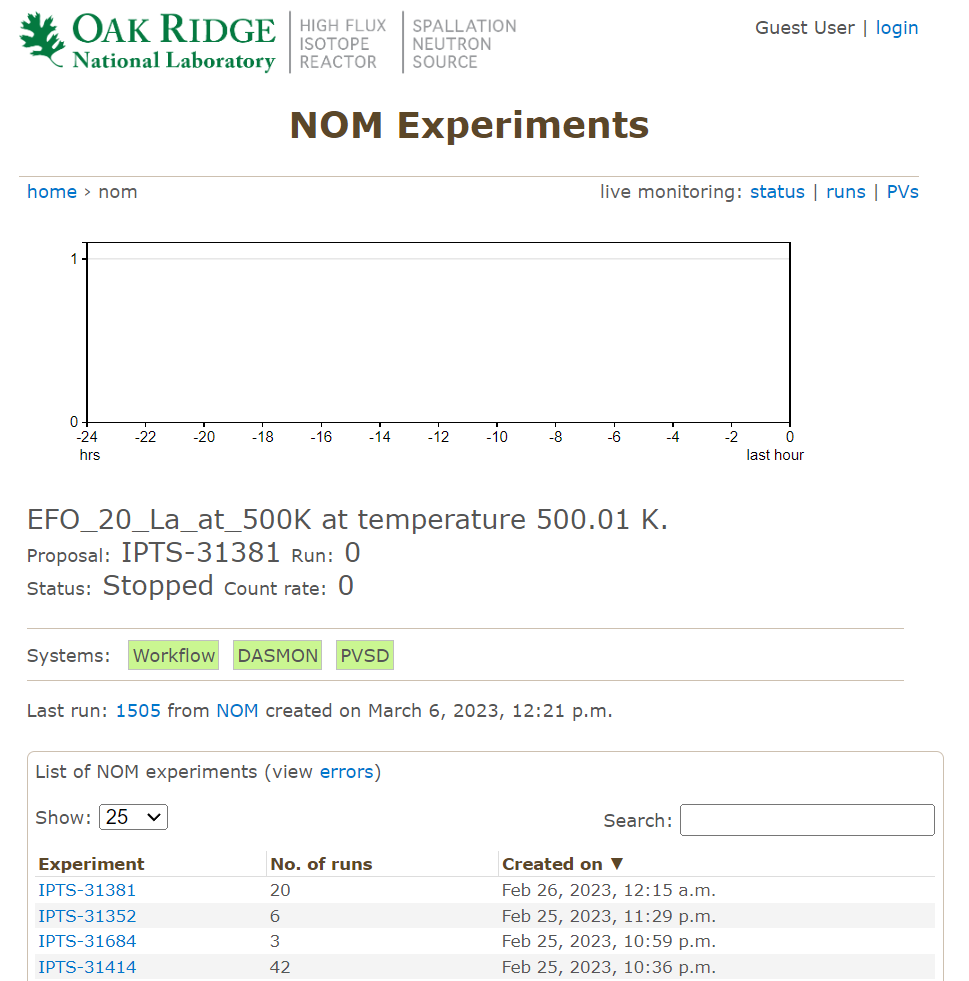
3. Click into an IPTS and you will see the list of runs,

   

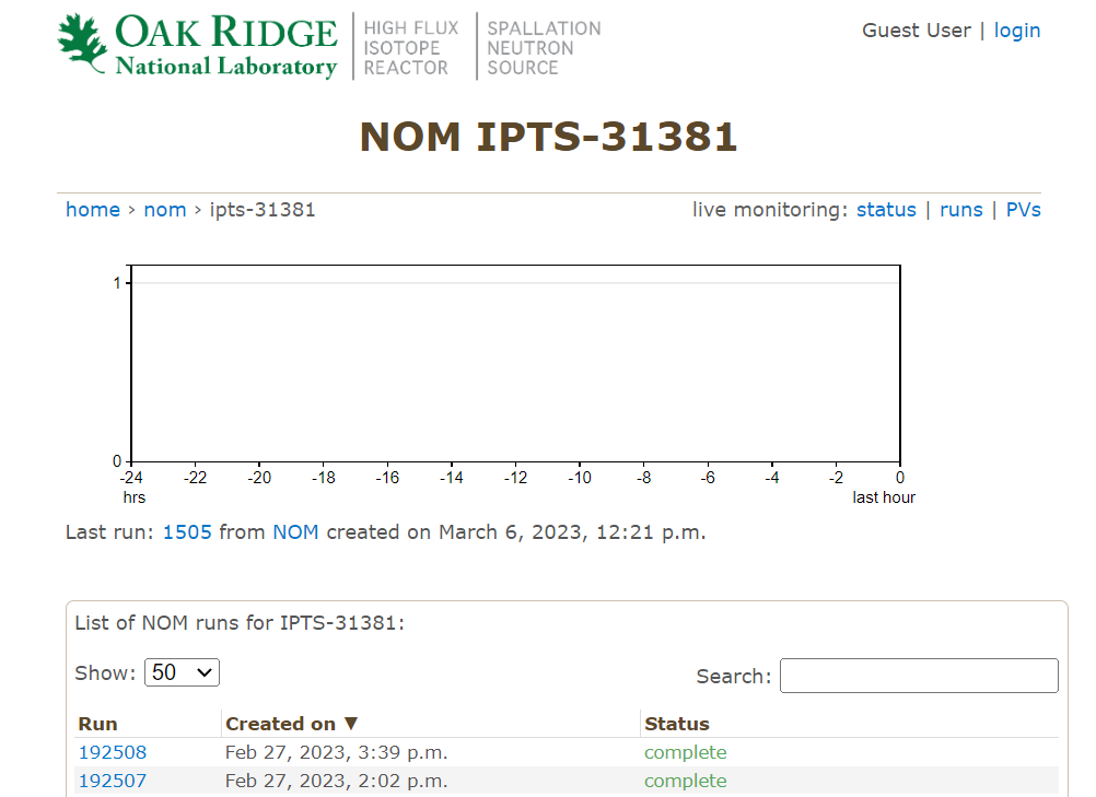
4. Scroll to the botom of the page, and find the reduction option,

   

5. Click on the link and the autoreduction will be kicked off.

6. For users with admin access, one can go to the top of the page and click on admin to see,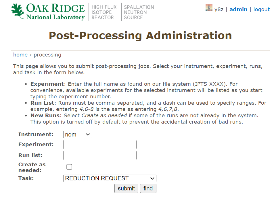

   

   where one can fill in necessary information and selection REDUCTION.REQUEST option from the dropdown menu to submit batch runs of autoreduction jobs.### Manual submission

Location of Files

Reduced Data

The reduced data from the auto-reduction routine will be saved to the IPTS specific autoreduce directory. Taking the IPTS-28922 example, the full path to the reduced data will be /SNS/NOM/IPTS-28922/shared/autoreduce. There are multiple sub-directories in autoreduce, with the following structure,

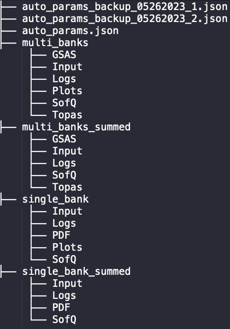
The single_bank and multi_banks directories are hosting the reduced data for each individual run, following the single-bank and the multi-banks mode, respectively. The single_bank_summed and multi_banks_summed directories are hosting the summed data for all similar runs, again, following the single-bank and the multi-banks mode, respectively. All those sub-directories should be self-explaining from their names. The Input sub-directory is worth mentioning – the input used for running either the individual or summed reduction is saved in the Input sub-directory for later tracking purpose.

Intermediate Files

This section may not be (and should not be) of interest to general users since it is more about the intermediate files that are saved when auto-reduction is running. In case of need, one could use those intermediate files for inspecting the issue when the auto-reduction encounters errors or unexpected behaviors.

First, both the absorption pre-calculation and the auto-reduction routine will access the absortion calculation cache files. For the commonly shared files among experiments, typically concerning the vanadium absorption correction, they can be found at /SNS/NOM/shared/mts_abs_ms. For the IPTS specific absorption cache files, they can be found at, e.g., /SNS/NOM/shared/mts_abs_ms/IPTS-28922, again, taking the IPTS-28922 as an example. Within the IPTS specific directory, the sample information file can also be found, in both JSON format (28922_sample_info.json, non-human-readable, and should only be used by the absorption calculation utility) and the CSV format (abs_calc_sample_info.csv, human-readable and configurable).

During the individual reduction runs, the align and focused data will be cached to the IPTS specific directory, e.g., /SNS/NOM/IPTS-28922/shared/autoreduce/cache. These files will be loaded in for both the summed run and also the potentially needed manual reduction later.

As mentioned in the introduction part, the auto-reduction routine will collect all the sum run configuration and accmulate them into a compact JSON file for the manual data reduction software ADDIE to load in. Such a JSON file will be saved to the autoMTS directory under the IPTS shared directory (e.g., /SNS/NOM/IPTS-28922/shared/autoMTS). Two JSON files will be saved to host the configuration for the single-bank and multi-banks mode of reduction, and the file name will be auto_sgb.json and auto_mtb.json, respectively.

Coder Notes

1. The autoreduction for various diffraction techniques at SNS and HFIR diffractometers have been re-vamped so that a consistent scheme of deveployment is applied across techniques. The design is to use the suitable conda environment for performing the reduction job, where the conda environment being used can be easily configured within the autoreduction script (as simple as specifying, e.g., CONDA_ENV = 'mantidtotalscattering-dev').

2. To test the autoreduction routine locally, one could grab the autoreduction script, make changes, and test it with the command,

   2.1. . /opt/anaconda/etc/profile.d/conda.sh && conda activate mantidtotalscattering-dev

   2.2. python /path/to/reduce_NOM.py /path/to/input/nexus /path/to/output/that/is/out/of/the/way