POWGEN | BL-11A | SNS#
Step-by-step Instruction#
…to be done
Advanced Setup#
This tab of the GUI is for hosting some advanced configurations for the data reduction, as can be glimpsed from the following snapshot,
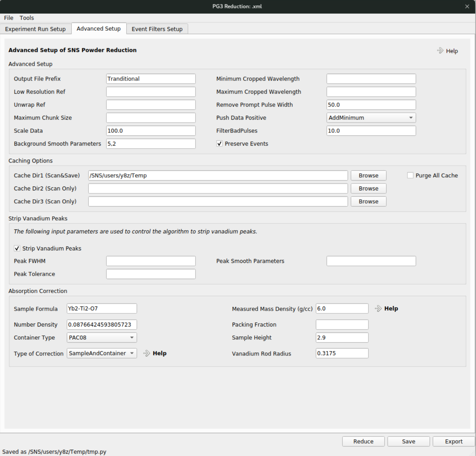
… Put items worth of special mentioning here …
Absorption Correction#
This section is for setting up the absorption correction, given some basic inputs about the sample under the beam. The required inputs are Sample Formula, Measured Mass Density, Container Type, and Type of Correction for general samples, together with the Vanadium Rod Radius for vanadium correction. The Sample Formula input should be following a certain format, typically like this,Yb2-Ti2-O7. The Measured Mass Density refers to literally the measured mass density given in g/cc. The Number Density refers to the theoretical number density of the sample, in the unit of \(Å^{-3}\) – it can be obtained from, e.g., a CIF file for the crystallographic structure of the sample. With both the Measured Mass Density and Number Density present, the Packing Fraction will be calculated and the corresponding box will be populated with the calculated value automatically - thus the input box for Packing Fraction is not editable. The Container Type dropdown menu is for specifying the geometry of both the container and the sample, which is needed for the absorption calculation. Instead of manual input for the geometry information (container inner, outer radius, and container height), a dropdown list is provided for all the typically used containers on POWGEN, where general users could select according to which of those containers were being used for their experiments. The Type of Correction dropdown is a list of alternative methods for the absorption correction. Here, details about those different methods will not be covered, and interested readers could refer to the documentation page located at https://docs.mantidproject.org/v6.5.0/concepts/AbsorptionAndMultipleScattering.html. The Vanadium Rod Radius entry is literally for providing the radius of the vanadium rod being used for normalization purpose. The Sample Height (given in cm) entry is optional – if it is not given, the program will try to read the value in from the sample log (embedded in the saved raw data of the measurement in NeXus format).
Here, it is also worth mentioning the Caching Options in the middle of the GUI interface presented above – it is for caching the absorption calculations. For a specific sample associated with specific geometry and among other configurations (which one would set up following the instruction above), the absorption calculation only needs to be performed once, and any further data reduction associated with the identical setup of the sample should be able to use the already performed absorption calculation. A typical use case is the absorption correction for a series of temperature measurement for the same sample, for which we should not repeat the absorption calculation which is computationally heavy. There are three input boxes for cache directory input. The first entry is for users to save and load their own version of the cache files. The second one should be an IPTS specific directory and it will be only used for loading (i.e., the absorption calculation will not be saved to that directory). Similarly we have the third entry, which should be a central place hosting the common absorption calculations. e.g., for vanadium, and again, this directory will only be used to load existing cache files. So, in practice, if we want to populate the specified second or third directory, we need to first run the normal reduction by specifying a save directory to host the calculated absorption in the first entry. Then, we need to copy the saved absorption cache file to either the second or the third directory. As a general user, one can copy the saved absorption cache file to their IPTS folder (under shared) and specify the corresponding directory path as the second entry. As an instrument team member, one should grab the saved absorption cache file (e.g., for vanadium) and put it somewhere under the instrument shared folder so that in the future general users can specify that central path as the third entry.
The absorption correction through the Advanced Setup GUI above applies to the situation where the normal container types are used for the measurement. By normal, we mean the standard vanadium container used on POWGEN with different specification, including QuartzTube03, PAC06, PAC08, PAC10 and PowderCell. The geometry definition for such standard container types can be found here. Selection of the container type being used can be made through the GUI presented above.
Coder Notes
Absorption Correction – Special Geometries#
When the container being used for the holding the sample is not one of those standard ones as defined in the Mantid code base (see the defined containers here), we have to perform the data processing using the scriptable interface of Mantid. Here I am providing a template for such a purpose below, with some notes about the setup.
from mantid.simpleapi import *

sam_geo = {
    'Shape': 'HollowCylinder',
    'Height': 4.0,
    'InnerRadius': 0.3,
    'OuterRadius': 0.32,
    'Center': [0.,0.,0.]
}

c_geo = {
    'Shape': 'HollowCylinderHolder',
    'Height': 4.0,
    'InnerRadius': 0.28,
    'InnerOuterRadius': 0.3,
    'OuterInnerRadius': 0.32,
    'OuterRadius': 0.34,
    'Center': [0.,0.,0.]
}

c_mat = {
    'ChemicalFormula': 'V',
    'NumberDensity': 0.072324
}

SNSPowderReduction(
    Filename='/SNS/PG3/IPTS-34523/nexus/PG3_58812.nxs.h5',
    CalibrationFile='/SNS/PG3/shared/CALIBRATION/2025-1_11A_CAL/PG3_OC_d58772_2025-02-12.h5',
    CharacterizationRunsFile='/SNS/PG3/shared/CALIBRATION/2025-1_11A_CAL/PG3_char_2025_2-HighRes_OC.txt,/SNS/PG3/shared/CALIBRATION/2025-1_11A_CAL/PG3_char_2025_2_OC_limit.txt',
    RemovePromptPulseWidth=50,
    Binning='-0.0008',
    BackgroundSmoothParams='5, 2',
    FilterBadPulses=90,
    ScaleData=100,
    TypeOfCorrection='SampleAndContainer',
    SampleFormula='Ba-Nb-Cr-Ru',
    MeasuredMassDensity='6.0',
    SampleGeometry=sam_geo,
    SampleNumberDensity='0.088',
    ContainerGeometry=c_geo,
    ContainerMaterial=c_mat,
    SaveAs='gsas topas and fullprof',
    OutputDirectory='/path/to/output/directory',
    CacheDir='/path/to/cache/directory'
)
Documentation for those parameters for SNSPowderReduction can be found here. Specifically concerning the geometry definition, one can see that we are basically using the SampleGeometry, ContainerGeometry and ContainerMaterial parameters. The former two defines the geometry for sample and container, respectively while the ContainerMaterial parameter defines the container material. For the geometry definition, the bottom-level Mantid algorithm SetSample is used and one can refer to the documentation here for available options. The one I presented above is for defining an annular container that sometimes will be used to, e.g., suppress the sample absorption. The length numbers involved in the geometry definition above are in cm. So, the sample defined above is a hollow cylinder with the thickness of 2 mm. The container holding the sample is an annular container with the wall thickness of 2 mm. The height for both sample and container is 4 cm. The Center entry for both definition means we want to put the sample and container as such that their geometrical center is located at [0, 0, 0]. By default, the orientation for both will be that the vertical axis of the geometry is lying along the y-axis – see the illustration for the coordinate system used in Mantid below,
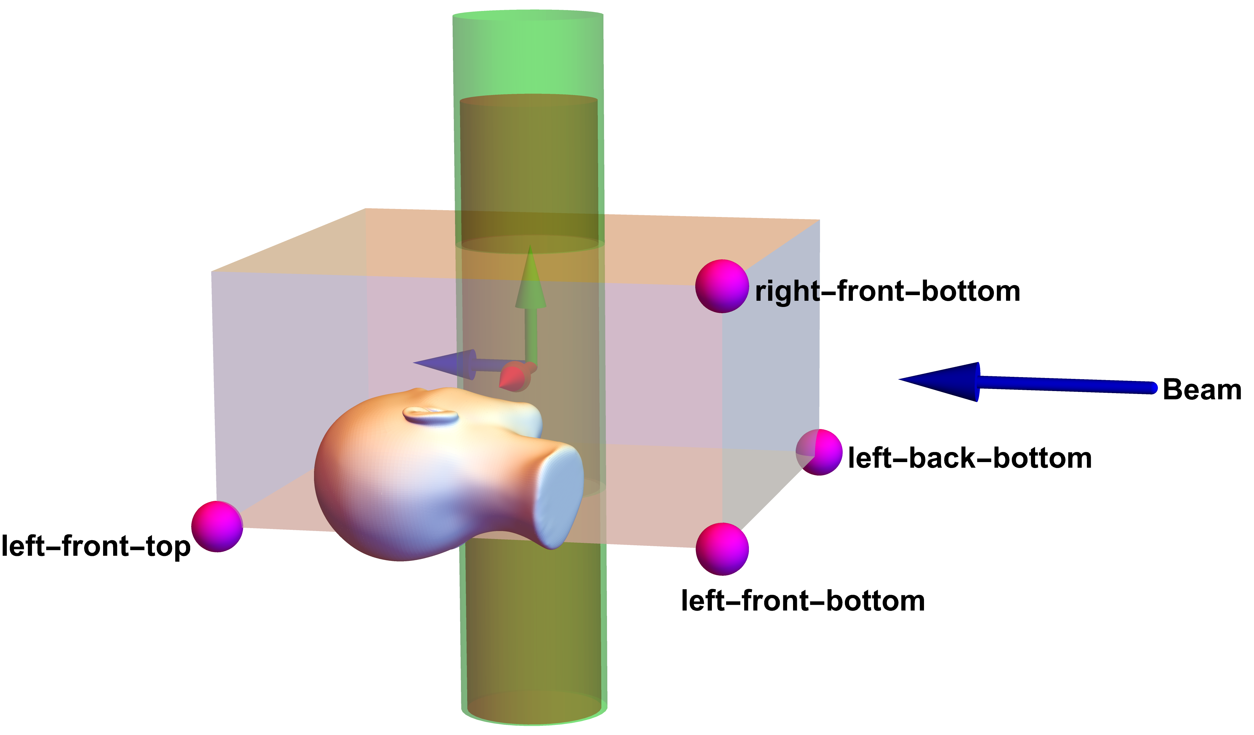
Image from the blog post by Yuanpeng Zhang – see the link here.
It is also worth mentioning that both the number density for sample (SampleNumberDensity) and container (NumberDensity in ContainerGeometry) refers to the full number density, i.e., assuming a full packing. Specification of the chemical formula can refer to the documentation here.
Absorption Correction – Account for Beam Size#
Till now, we have been assuming that the beam size is the same as the sample size for the absorption correction purpose, which in practice is quite often not true. The beam size can be accounted for, by defining the so-called gauge volume in Mantid, which basicaly defines the region of the sample and container that is exposed to the incident beam, i.e., where the single scattering events are supposed to happen. For such a purpose, I am sharing an example below, with some notes.
from mantid.simpleapi import *
import matplotlib.pyplot as plt
import numpy as np

SNSPowderReduction(
    Filename='/SNS/PG3/IPTS-34523/nexus/PG3_58812.nxs.h5',
    CalibrationFile='/SNS/PG3/shared/CALIBRATION/2025-1_11A_CAL/PG3_OC_d58772_2025-02-12.h5',
    CharacterizationRunsFile='/SNS/PG3/shared/CALIBRATION/2025-1_11A_CAL/PG3_char_2025_2-HighRes_OC.txt,/SNS/PG3/shared/CALIBRATION/2025-1_11A_CAL/PG3_char_2025_2_OC_limit.txt',
    RemovePromptPulseWidth=50,
    Binning='-0.0008',
    BackgroundSmoothParams='5, 2',
    FilterBadPulses=90,
    ScaleData=100,
    TypeOfCorrection='SampleAndContainer',
    SampleFormula='Ba-Nb-Cr-Ru',
    MeasuredMassDensity='6.0',
    SampleGeometry={
        'Height': 5,
        'Radius': 0.295
    },
    BeamHeight=2,
    SampleNumberDensity='0.088',
    ContainerShape='PAC06',
    ContainerGaugeVolume='0.295 0.315',
    SaveAs='gsas topas and fullprof',
    OutputDirectory='/path/to/output/directory',
    CacheDir='/path/to/cache/directory'
)
Here we are defining the gauge volume internally in Mantid and the interface to users is BeamHeight (in cm). In fact, it is the intersection part between the internally defined beam volume and the samplethat gives the gauge volume – refer to the illustration diagram above. The beam volume geometrical center is assumed to be at the origin. Following the same logic, we can define the gauge volume for the container as well – the ContainerGaugeVolume parameter gives the inner and outer radius of the container. Together with the BeamHeight parameter, they will together define the container gauge volume internally in Mantid.
In fact, programmingly the
gauge volumecan be figured out automatically using theSetBeamalgorithm internally in Mantid so that we don’t need to specify either the sample or containergauge volume. We also don’t even need to set up thegauge volumein the Mantid code base explicitly either –SetBeamwill automatically figure out the intersection region between the beam and sample/container. This is indeed the case for theTypeOfCorrection='FullPaalmanPings'type of absorption correction.
If we want more flexibility in defining the gauge volume, we can refer to the following example,
from mantid.simpleapi import *

sam_geo = {
    'Shape': 'HollowCylinder',
    'Height': 4.0,
    'InnerRadius': 0.3,
    'OuterRadius': 0.32,
    'Center': [0.,0.,0.]
}

c_geo = {
    'Shape': 'HollowCylinderHolder',
    'Height': 4.0,
    'InnerRadius': 0.28,
    'InnerOuterRadius': 0.3,
    'OuterInnerRadius': 0.32,
    'OuterRadius': 0.34,
    'Center': [0.,0.,0.]
}

c_mat = {
    'ChemicalFormula': 'V',
    'NumberDensity': 0.072324
}

gauge_vol = """<hollow-cylinder id="sample_gauge">
    <centre-of-bottom-base r="1.0" t="180.0" p="0.0" />
    <axis x="0.0" y="1.0" z="0.0" />
    <inner-radius val="0.3" />
    <outer-radius val="0.32" />
    <height val="2.0" />
    </hollow-cylinder>
"""

SNSPowderReduction(
    Filename='/SNS/PG3/IPTS-34523/nexus/PG3_58812.nxs.h5',
    CalibrationFile='/SNS/PG3/shared/CALIBRATION/2025-1_11A_CAL/PG3_OC_d58772_2025-02-12.h5',
    CharacterizationRunsFile='/SNS/PG3/shared/CALIBRATION/2025-1_11A_CAL/PG3_char_2025_2-HighRes_OC.txt,/SNS/PG3/shared/CALIBRATION/2025-1_11A_CAL/PG3_char_2025_2_OC_limit.txt',
    RemovePromptPulseWidth=50,
    Binning='-0.0008',
    BackgroundSmoothParams='5, 2',
    FilterBadPulses=90,
    ScaleData=100,
    TypeOfCorrection='SampleAndContainer',
    SampleFormula='Ba-Nb-Cr-Ru',
    MeasuredMassDensity='6.0',
    SampleGeometry=sam_geo,
    SampleNumberDensity='0.088',
    ContainerGeometry=c_geo,
    ContainerMaterial=c_mat,
    GaugeVolume=gauge_vol,
    SaveAs='gsas topas and fullprof',
    OutputDirectory='/path/to/output/directory',
    CacheDir='/path/to/cache/directory'
)
Here the gauge volume is defined explicitly as gauge_vol with an XML string. It should be noticed that the length and angle unit for the XML geometry definition is m and degree, respectively. Refer to the link here for more information.