Calibration assessment, completion and output

Calibration assessment, completion and output#

At present, graphical inspection of calibration output is achieved via inspection of workspaces within mantid workbench. The output of a typical calibration is shown in Figure

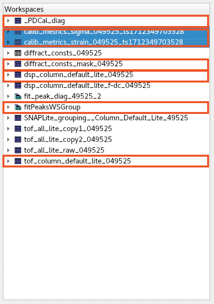
../../../../_images/outputWS_cisModeFalse.png — Fig. 3 The mantid workbench workspace tree with useful workspaces indicated.#

Diffraction focused data#

At this stage in diffraction calibration, the resultant set of diffractometer coefficients, generated via the two step pixel and group calibration approach, $\mathbf{C^{CC,PD}}$ have to be assessed. This is done by applying them to the input data (Mantid algorithm ApplyDiffCal) and then diffraction focusing (using the specified PGS).

The resultant spectra are available in the mantid workspace tree to inspect, which will have the name:

dsp_{pixel grouping scheme}_{run number}

These can be compared with earlier calibrations from the same state, allowing comparisons of different calibration approaches and different calibrants. If an earlier calibration exists, it can be loaded by selecting from the Calibration Record drop down on the assessment tab. Loading an earlier calibration will load it’s set of diffraction focused data (focused using the applied pixel grouping scheme) and its calibration metric workspaces (see below)

Calibration Mask#

Another useful workspace to inspect is the mask file, which has the name

diffract_consts_mask_{run number}

You can expand the workspace to inspect the number of masked pixels, ideally this will be zero, but a small number of masked pixels is not uncommon. If there are many masked pixels, it likely indicates something is wrong. You can right click on the workspace and select Show Instrument to look for geometric patterns that may help diagnose issues.

Metrics#

It is helpful to have a simple metric that allows rapid assessment of calibration quality and comparison between calibrations. This is done fitting the diffraction focused data - using a Gaussian peak shape - to extract peak position and widths (the latter estimated via the Gaussian standard deviation). These are used to calculate two parameters:

“strain” this is $\frac{1}{N_{hkl}}\sum_{hkl}\frac{d^{obs}_{hkl}-d^{calc}_{hkl}}{\sigma_{hkl}}$ for each subgroup. Thus, this captures the average deviation from the correct d-spacings in each group, as a fraction of the gaussian standard deviation $\sigma_{hkl}$ of each peak. A smaller absolute valuer is better.
“sigma” this is $\frac{1}{N_{hkl}}\sum_{hkl}\frac{\sigma_{hkl}}{d_{hkl}}$ for each subgroup. This captures something that approximates an average $\frac{\delta d}{d}$ for the subgroup, smaller is better.

The resultant two values are captured for each group in the PGS as a function of scattering angle %2\theta$ in workspaces with names similar to these (for calibrant run 57474):

calib_metrics_sigma_057474_ts1711137415314
calib_metrics_strain_057474_ts1711137415314

Here the final part of the workspace name is a time stamp. SNAPRed allows the calibration process to be repeated iteratively allowing, the optimal calibration to be accepted (n.b. at present - in Phase 2 - a calibration is not propagated from one interation to the subsequent one, so not truly iterative. This is planned to be fixed.).

It is also possible to compare these metrics with earlier completed calibrations for the same state, allowing a more global assessment of quality between calibrations conducted at different times, or for different calibrant materials.

When a calibration is finalised, these metrics are saved as part of the calibration record and can be reloaded for comparison between different calibrations.

Note

Plotting these parameters vesus 2$\theta$ works well for pixel groups at non-overlapping angles. However, this is not so clear where these overlap (e.g. when both detectors are at 90° there is 100% overlap of pixel group angles between the two banks). Addressing this may be possible with a customised GUI.

Detailed inspection: Group Calibration#

During Group Calibration, a set of peaks is fitted in each pixel group using mantid algorithm PDCalibration. The resultant fits are stored in the workspace _PDCal_diag, these are in TOF and can be compared with the corresponding input data, which are stored in `tof_{pixel grouping scheme}_{run number} using the plot spectrum option in workbench.

Meanwhile, the corresponding fit parameters are stored in a grouped workspace fitPeaksWSGroup. These contain table workspaces with names fitPeaksWSGroup_fitted_params_{n} for each pixel group (note $n$ is the spectrum index, which is groupID-1). In addition to the parameters, a $\chi^2$ is reported, a graphic interface for this has been developed, whereby a grid of plot axes shows the data and fitted spectra for each group and indicates peaks with $\chi^2$ above a threshold value of 100 by colouring these red.

Note

In testing it was noticed that very high $\chi^2$ values can be found for long datasets. This is due to random errors due to Poisson counting statistics becoming very small relative to systematic errors from using incorrect peak shape (at present, PDCalibration can only use symmetric peak models, which do not perfectly fit the TOF peakshape).

Modification of the threshold value of $\chi^2$ can be achieved via editing `application.yml. This allows calibration to continue with for these longer datasets

Detailed inspection CIS mode#

More detailed diagnostic information is accessible by through the cis_mode option. This is currently accesible in the application.yml and, if set True will preserve intermediate workspaces, which can be inspected.

The values of the calculted offsets are stored in workspaces with the name offsets_{run number}_{iteration}. These contain the value of the offset (in units of absolute number of bins)for every pixel and can be inspected using either the Plot/Bin or Show Instrument methods to look for geometric trends. In particular, the maximum offset is currently hardwired to not exceed 10: if multiple spectra have offsets equal to this hard limit, it likely indicates an issue with the input data.

The workspace DSP_{run number}_diffoc_before shows the diffraction focused dataset prior to Group Calibration and can be used to inspect the effect of that latter but comparing with the final output: dsp_{pixel grouping scheme}_{run number}.

Diffraction calibration outputs#

When satisfied with the results of the calibration, the resultant output is saved to disk:

a set of calibrated diffractometer constants stored in an mantid diffcal .h5 file (this includes the calibration mask)
a calibration record capturing all other parameters from the calibration.
a copy of the “strain” and “sigma” metrics and final diffraction-focused dataset.

It is also required that the user specify to which run number the calibration applies from. This defaults to the run number of the diffraction calibrant however, it can be specified to an earlier run number (for example when a calibration is conducted after a sample dataset was measured). This is then stored in the calibration index for the state to allow for the automatic location of the appropriate calibration to be used when reducing sample data.