Diffraction Calibration

The goal of Diffraction Calibration

Powder diffraction measurements embody a rich source of information on the atomic structure of the sample of interest. The presence and position of Bragg peaks encode information on the crystallographic unit cell (and the effects of any stress it is under). The intensity of the peaks encode the details of the nuclear density within the unit cell convolved with the orientational distribution of the sample crystallites, while the width and shape of the Bragg peaks encode details of sample strain fields, particle size and shape [C.J. Gilmore, 2009].

As these properties of Bragg peaks are also modified by purely instrumental artifacts,the goal of calibration measurements is determine these fully, in order to deconvolve those effects from the sample measurement. The process of diffraction calibration has two main goals: to determine the relationship between crystallographic d-space and measured time-of-flight of detected neutrons and to fully quantify the native peak width and shape of the instrument.

This section specifies the process used by SNAPRed for the former goal. The latter goal is captured via separate workflows currently using external Rietveld packages, such as GSAS [Larson and Dreele, 2004].

Inputs

The inputs to Diffraction Calibration are:

1. A set of neutron powder diffraction data from a known calibrant material, measured in a given instrument state. This is specified via its run number.

2. Crystallographic information on the calibrant material (see below).

3. A pixel grouping scheme (e.g. Column or any arbitrary scheme) that is used during calibration (as described below), but does not impose any constraint on any subsequent choice of grouping used during reduction.

4. A set of parameters governing the calibration workflow. Some of these are fixed and some are variable. The ultimate goal is to fix everything possible to fully automate the calibration process.

A note on input data: Despite it’s best efforts, SNAPRed will always be limited to the quality of the input calibration data. Known issues have been observed under the following circumstances:

• Input data with insufficient counting statistics. both components of the diffraction calibration workflow include execution of algorithms that will fail if input data are too noisy.

• Calibrant sample too far off instrument centre. initial guesses for peak positions will fail if the physical location of the calibrant sample is too far away from the nominal instrument centre. Best practice is to identify the instrument centre and deploy aligment approaches guaranteed to repeatedly position the calibrant sample in this absolute location.

• Crystallographic properties of calibrant. SNAPRed uses the mantid alogrithm PDCalibration, which is limited to fitting isolated peaks. At least two non-overlapping peaks in every pixel group are required for it to run.

• Input data with poor signal-to-background the pixel calibration requires the determination of a peak centre from a cross-correlation, which can become unreliable for high-background data.

Overall methodology

The basic approach is to use the diffraction signal from a known calibrant material in order to establish the relationship between the measured variable of time-of-flight and the crystallographic parameters of the calibrant. SNAPRed borrows the diffraction calibration methodology from an existing approach, developed for POWGEN and NOMAD. This approach consists of two operations:

1. Make the diffraction-focused peaks as sharp as possible

2. Make the resulting (sharp) peaks positions (as ascertained via a specified peak fit) match as closely as possible the correct d-spacing

The first step is referred to as “pixel calibration”, the second step “group calibration”. The word group calibration implies the existence of a “Pixel Grouping Scheme”, this is nothing other than an assigned grouping ID to SNAP pixels. For example, grouping can be defined according to detector components (such as “Banks” or “Columns”), but SNAPRed is not limited to this and can calibrate with any arbitrary grouping definition

The pixel grouping scheme is chosen by the user at the onset of the Diffraction Calibration workflow.

Calibrant samples.

The choice of calibrant sample is fundamental to the calibration measurement. For example, any uncertainty in the absolute values of the calibrant lattice parameter will propagate - via the diffractometer constants - into error in the subsequent measurement of any sample that uses that calibration. Similarly, the use of calibrant samples with intrinsic strain, or small particle sizes will interfere with accurate characterisation of the native instrumental peak shape. An additional consideration is the range of d-spaces to be study, which on SNAP is highly variable, depending on instrument state.

For these reasons, SNAPRed uses an established library of calibrant samples. Each calibrant sample is represented by a json file containing relevant information on the sample including its crystal structure (and a citation to the source of this information), and its geometry, material and nuclear properties. Each calibrant has a unique ID and an easily readable name.

A future goal is to record the calibrant within the experimental process variable logs via use of RFID tags.

Essential background theory

A sufficient theoretical background to follow diffraction calibration process is obtained from Bragg’s Law:

\(\lambda = 2d\sin\theta\)

where \(d\) is a d-spacing corresponding to the separation of a particular set of cystallographic planes (labelled by Miller indices \(hkl\)) and \(\theta\) is half of the scattering angle, and the deBroglie relation for non-relativistic neutrons:

\(\lambda = \frac{h}{p_n}\)

Here \(p_n\) is the neutron momentum, which is given by the product of the neutron mass (\(m_n\)) and its velocity (\(v_n\)). A neutron travelling at a constant velocity will traverse a known pathlength \(L\) in a time \(T\). For neutrons at a pulsed source, it is possible to measure \(T\) as the “time-of-flight” between neutron generation and detection.

By substituting this above and equating the two equations, we see that a given Bragg peak with indices \(hkl\) will be observed at a corresponding time of flight \(T^{hkl}\) given by:

\(T_{hkl}=(\frac{2m_n}{h})L\sin\theta d_{hkl}\)

For any given pixel, \(i\), this can be written as

\(T_{hkl,i}=C_i d_{hkl,i}\)

Where \(C_i=(\frac{2m_n}{h})L_i\sin\theta_i\) is a constant for pixel i at fixed scattering angle \(2\theta_i\) and for which a detected neutron will have traversed a total distance of \(L_i\) after scattering from the sample.

In general, details including the finite thickness of the neutron source (a moderator) and time offsets between proton pulse and neutron generation require a more complex relation where the relation from between \(T^{hkl}\) and \(d^{hkl}\) is parabolic, follow the definition in the GSAS manual [Larson and Dreele, 2004].

\(T_{hkl,i}=A_i {d_{hkl,i}}^2 + C_i d_{hkl,i} + Z\)

And the set of values \(A_i\), \(C_i\) and \(Z\) are called the diffractometer constants, specified as arrays for each of the \(N_{pix}\) pixels.

However, at present, SNAPRed calibration is based on the approximation \(T_{hkl}=C_i d_{hkl,i}\).

Diffraction Calibration part 1: pixel calibration

The first step of diffraction calibration, Pixel Calibration, is based on the mathematical process of cross correlation (CC) between the data in a reference pixel and adjacent pixels. In SNAPRed, this is governed by the selected Pixel Grouping Scheme. For example, if “Column” grouping is selected, the algorithm will progress through each of the corresponding 6 pixel groups (one for each detector column). In each group, a reference pixel is selected (ensuring that this is always the same pixel for every group in a given pixel grouping scheme), and then the diffraction data in every other pixel in the group is cross-correlated against that of the reference.

Prior to the cross-correlation calculation, input data that are measured as a function of TOF are converted to d-spacing (this is currently done using the default instrument definition, but will be extended to use any pre-existing calibration) and histogrammed, using a logarithmic binning scale. Logarithmic binning is essential to enable to full-pattern cross correlation conducted by SNAPRed, discussed below. The selection of binning parameters occurs automatically, with SNAPRed selecting values that are appropriate for the relevant instrument state and selected pixel group.

The cross-correlation itself is conducted using the mantid algorithm CrossCorrelate. The operation is a way to identify how similar two signals are as a function of their offset relative to each other along a shared x-axis. In our case, the input data are histogrammed neutron counts versus d-spacing.

Since the input spectra contain sharp Bragg peaks all at the same d-spacings, the CC will also have a sharp peak. In a perfectly calibrated instrument, the Bragg peaks in any spectra should occur at the same d-spacings and the CC peak would be centred on an offset of zero. However, if errors in calibration are present, they will cause this peak to shift from zero by a certain number of d-space bins, \(N^{off}\). By correcting for this non-zero offset, we obtain optimal agreement between the observed d-spacings in every pixel.

An important advantage of the CC approach is that it is independent of any assumption of peak shape and a reliable CC signal can be obtained even when the input data are rather noisy (especially when using whole-pattern cross correlation). This is a significant boon when trying to minimise data collection time needed for calibration.

In real data, the Bragg signal will be combined with experimental background that (normally) will be broadly varying as a function of d-spacing. This background propagates into the CC with the corollary that the algorithm will work better for high signal-to-background input data (n.b. During testing, specific issues were observed with input silicon powder data measured in a kapton container). It is intended that SNAPRed will calculate and subtract a background prior to CC calculation, but this feature isn’t yet available.

Determining the offset

Once the CC has been obtained, a second step is to determine the centre of the sharp CC peak corresponding to the value of offset (\(N^{off}\)), that maximises the overlap of the diffraction data in the two spectra. Again, SNAPRed uses a mantid algorithm GetDetectorOffsets, which performs peak fitting to extract a peak centre of the CC to return (\(N^{off}\)). SNAPRed currently uses a Gaussian peak shape to fit the CC. GetDetectorOffsets will create a workspace of offsets, containing a the numerical value of the determined offset for each pixel.

Once CC has executed across all pixel groups, and (\(N^{off}_i\)) has been determined for every pixel \(i\), the final step in pixel calibration is to apply this to the initial values of the diffractometer constants \(C_i\) used to convert each i from TOF to d-spacing. This calculation is conducted by the mantid algorithm ConvertDiffCal and returns a new set of \(C_i\) values that include the offset correction.

Single peak cross correlation

The most common approach when conducting cross-correlation while calibrating a TOF diffractometer is to select a single Bragg peak. This peak must be common to all pixels within the group of pixels that are being cross correlated.

In such a calculation, it is appropriate that the input data are a function of d-space and have linear binnning with step size \(\Delta d_{lin}\). The resultant applied CC correction corresponds to an additive shift of the x-values by \(N^{off}_i \Delta d_{lin}\) of the input data for pixel \(i\) to maximise overlap with the data in the reference pixel.

The offset is currently managed in Mantid by replacing the initial diffractometer constant \(C^{init}_i\) by a new constant \(C^{CC}_i\) that includes the offset correction. This immediately creates consideration that the diffractometer constants are applied by multiplication versus in contrast to an offset, which is additive (a shift of the histogram of y-values along the x-axis by \(N^{off}\) bins). These two distinct operations can only agree at a single point in d-space, \(d'\) (see Figure).

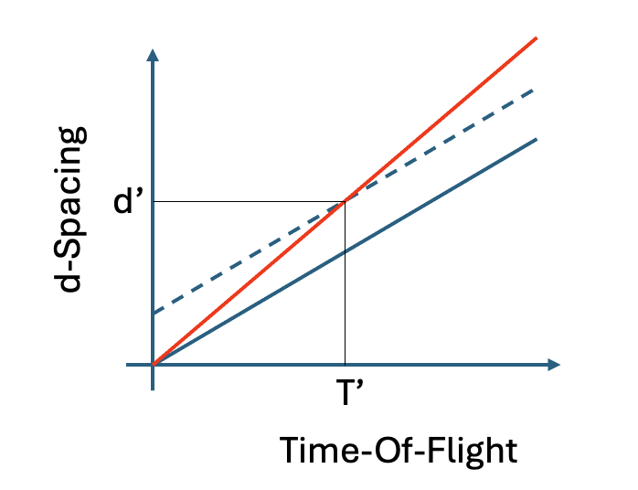
Fig. 1 The solid blue line shows the initial relationship between \(\mathbf{T}_i\) and \(\mathbf{d}_i\) for pixel \(i\): a straight line with gradient \(\frac{1}{C^{init}_i}\). Instead of applying an additive offset, which would shift the all values of d by a constant (as indicated by the dashed blue line), the CC-corrected diffractometer constant \(C^{CC}_i\) must be calculated by considering the offset at a specific d-value \(d'\), using this to calculate the gradient of the red line, which gives the new \(C^{CC}i\).

To enable this, a value for \(d'\) (typically the expected d-spacing of the chosen Bragg peak) must be specified when calling the mantid algorithm GetDetectorOffsets and, from this, the corresponding corrected diffractometer constant \(C^{CC}_i\) can be obtained. This calculation is supported by chosing the Relative Offset output mode of GetDetectorOffsets.

Whole pattern cross correlation

SNAPRed adopts a different approach, whereby the entire pattern is cross correlated. This utilises the counts from all present Bragg peaks, reducing the necessary collection time by a factor of 2-3, which is important for the frequent recalibrations necessary on SNAP.

This approach hinges on ensuring that the input diffraction data for each pixel have been binned \(logarithmically\). Due to the property of a TOF diffractometer that the diffraction resolution \(\delta d/d\) is approximately constant for a given detector, logarithmic binning ensures that each Bragg peak is (approximately) sampled with the same number of histogram bins. Consequently, intensity from each Bragg peak in the pattern will contribute to the total CC peak according to its own intensity.

Since the cross-correlation is not conducted using a single peak, there’s no obvious way to select a \(d'\) to scale the offset. However, this issue is also solved by log binning. This is seen from the (mantid) definition of log binning, where successive bin edges are related by the corresponding binning parameter is \(\Delta d_{log}\) according to:

\(d_{j+1}=d_j(1+\Delta d_{log})\)

and, the \(j^{th}\) d value can be calculated from the constant initial d value, \(d_0\) via

\(d_j = d_0(1+\Delta d_{log})^n\)

In this case, the CC offset of of \(N^{off}_j\), is applied in the exponent:

\(d_j^{CC} = d_0(1+\Delta d_{log})^{(n+N^{off}_j)}\)

This is equivalent to a multiplication and so the extracted \(N^{off}_i\) can be used directly to scale the diffractometer constants. This will be returned by GetDetectorOffsets by choosing the \(signed\) output mode.

Masking

A mask is automatically created for any pixels where the cross-correlation operation fails. This mask is persisted to disk as a property of the calibration and, subsequently, these pixels will not be included in data reduction using that calibration. During the calibration process, it’s important to inspect the output mask to identify pathlological issues (high background in the input data, for instance) with cross correlation that have been observed to lead to large numbers of pixels being masked.

Iteration

After running CrossCorrelation and GetDetectorOffsets, every pixel for which these operations have been successful will have a numerical value of the measured offset, stored in an offsets workspace. The next step is to apply these offsets via an operation that returns the corrected set of diffractometer constant for each pixel \(\mathbf{C}^{CC}\). This is done using the mantid algorithm ConvertDiffCal noting that SNAPRed returns offsets using the “Signed” mode. Subsequently, the set of CC-corrected diffractometer constants \(\mathbf{C}^{CC}\), are then applied to the input data set (Mantid algorithm ApplyDiffCal). If the data are then converted from the measured TOF to d-space (Mantid algorithm ConvertUnits) the Bragg peaks in each pixel within a specific subgroup will all have been offset towards same d-value, equal to that of the corresponding reference pixel.

At this point, SNAPRed will repeat the cross-correlation to try to further improve agreement between pixels. Since a cross-correlation has already been applied, the offsets calculated in a subsequent operation should be smaller than those in the preceding interation. These operations will continue until a specified Convergence Threshold is reached, which is defined as the average offset of pixels in the group (in units of number of bins) or until a maximum number of iterations (default is 10) is reached.

Warning

If convergence is not achieved before the maximum number of iterations is reached, it is likely there is a problem with your input data (e.g. low signal to background) and the final values of offsets may not be correct.

Cross correlation completion

Once optimised values for the offsets, and corresponding DIFC’s, have been determined, these should ensure that all common Bragg peaks in any spectrum in the group will have the same d-spacing values as the reference spectrum. However, these values may still be incorrect, due to any present (and unknown) offset of the reference pixel. This necessitates the second step of the diffraction calibration process: group calibration.

Diffraction Calibration Part 2: Group Calibration

The input data for Group Calibration is a diffraction focussed (Mantid algorithm DiffractionFocusing), using the CC-corrected diffractometer constants, and applying the specified pixel grouping scheme (PGS). This process combines the neutron counts in all pixels in each group into a single spectrum, reducing the total number of spectra in the dataset to the number of sub groups in the PGS, \(N_{grp}\). Due to the application of the cross correlation correction, the Bragg peaks in each diffraction-focussed group should be as sharp as possible, however, the absolute value of their d-spacings will, in general, still be incorrect. This is dealt with using a process of Group Calibration which employs the mantid algorithm PDCalibration applied independently for each subgroup in the PGS. The output of this process is a complete set of diffractometer constants that ensure the sharpest possible peaks at the correct positions in d-space.

The approach applied by PDCalibration is to fit the Bragg peaks in each input spectrum. This works well on the focussed dataset as the statistical quality of the data in each \(focused\) spectrum are much better than in individual pixels.

PDCalibration fits the data as a function of TOF and unit conversion must be done on the diffraction focused data prior to input into the algorithm. It operates by conducting a series of individual peak fits and, thus, has a requirement that the peaks selected for fitting do not overlap. To enable this, SNAPRed orchestrates the peak fitting in the following way for each pixel group:

• The peak positions in d-spacing are calculated for the calibrant sample via the user-selected cif file. The resultant list is truncated between the limits of the minimum and maximum d-spacings accessible to each pixel group, which SNAPRed calculates, respecting both the grouping scheme and the instrument state. Bragg peak intensity is estimated approximately by applying the TOF-powder specific Lorentz correction to the calculated structure factors squared and weak peaks can then be removed via a user-specified threshold (\(I_{thresh}\)) entered as a percentage of the estimated intensity of the strongest calibrant Bragg peak.

• The peak extents are estimated by first calculating the FWHM of each peak to be fitted - deriving this from the known diffraction resolution, respecting the pixel group properties and the instrument state. Second, the exponent of the exponential trailing edge tail of the TOF Bragg peak shape is determined. This latter follows the same parameterisation used by the GSAS TOF Peak Profile Function 3 [Larson and Dreele, 2004], whereby the exponent \(\beta\) is determined from its parameterised d-space dependence, converted to its equivalent in d-space \(\beta_d\) and the corresponding 1/e length calculated. These calculated values are then used to define a left and right extent (\(E_L\) and \(E_R\) respectively) by applying three multipliers (constants fixed for the instrument): \(M_{FWHM-L}\), \(M_{FWHM-R}\) and \(M_{tail}\) in the following way:

  \(E_L = FWHM*M_{FWHM-L}\)

  \(E_R = FWHM*M_{FWHM-R}+M_{tail}/\beta _d\)

• Using the calculated peak extents, the list of peaks is purged of any peaks that overlap. Since the calculation respects the varying (angular-dependent) diffraction resolution, different peaks may be purged in different groups. At least two peaks per group are required for PDCalibration to execute, but a larger number of peaks are recommended.

Prior to execution, the user is able to fine tune the list of peaks by adjusting the minimum and maximum d-spacing of the list and the peak intensity threshold \(I_{thresh}\). SNAPRed provides a visualisation of data and peak extents to support optimising the peak list prior to execution of group calibration.

Note

An idea, not yet implemented, is to record the optimal settings for each calibrant in its .json file. This will further automate the calibration process. At present there’s insufficient knowledge of what the best settings are, not how these vary with PGS and instrument state.

Lastly, the user is allowed the possiblity to select a peak shape. At present, due to a limitation of PDCalibration only symmetric shapes are supported: Gaussian, Lorentzian and psuedoVoigt. This is a known limitation but the best solution isn’t yet settled as use of asymmetric peak shapes will have additional impacts on subsequent analysis of reduced data (see here (to do)).

PDCalibration executes by fitting all of the specified peaks in each pixel group. This provides a set of pairs of \(T_{hkl}:d_{hkl}\) values (where \(d_{hkl}\) are known for the reference calibrant material) that can be used to determine the “correct” diffractometer constant \(C^{CC,PD}_j\) for the \(j^{th}\) group. Since - post cross correlation correction - all pixels in the group have their peaks at the same d-spacings, multiplying each diffractometer contant by the ratio \(\frac{C^{CC,PD}_j}{C^{CC}_i}\) will shift the peak for every pixel to the correct d-spacing.

Calibration assessment, completion and output

At present, graphical inspection of calibration output is achieved via inspection of workspaces within mantid workbench. The output of a typical calibration is shown in Figure

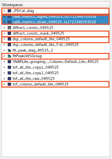
Fig. 2 The mantid workbench workspace tree with useful workspaces indicated.

Diffraction focused data

At this stage in diffraction calibration, the resultant set of diffractometer coefficients, generated via the two step pixel and group calibration approach, \(\mathbf{C^{CC,PD}}\) have to be assessed. This is done by applying them to the input data (Mantid algorithm ApplyDiffCal) and then diffraction focusing (using the specified PGS).

The resultant spectra are available in the mantid workspace tree to inspect, which will have the name:

dsp_{pixel grouping scheme}_{run number}

These can be compared with earlier calibrations from the same state, allowing comparisons of different calibration approaches and different calibrants. If an earlier calibration exists, it can be loaded by selecting from the Calibration Record drop down on the assessment tab. Loading an earlier calibration will load it’s set of diffraction focused data (focused using the applied pixel grouping scheme) and its calibration metric workspaces (see below)

Calibration Mask

Another useful workspace to inspect is the mask file, which has the name

diffract_consts_mask_{run number}

You can expand the workspace to inspect the number of masked pixels, ideally this will be zero, but a small number of masked pixels is not uncommon. If there are many masked pixels, it likely indicates something is wrong. You can right click on the workspace and select Show Instrument to look for geometric patterns that may help diagnose issues.

Metrics

It is helpful to have a simple metric that allows rapid assessment of calibration quality and comparison between calibrations. This is done fitting the diffraction focused data - using a Gaussian peak shape - to extract peak position and widths (the latter estimated via the Gaussian standard deviation). These are used to calculate two parameters:

• “strain” this is \(\frac{1}{N_{hkl}}\sum_{hkl}\frac{d^{obs}_{hkl}-d^{calc}_{hkl}}{\sigma_{hkl}}\) for each subgroup. Thus, this captures the average deviation from the correct d-spacings in each group, as a fraction of the gaussian standard deviation \(\sigma_{hkl}\) of each peak. A smaller absolute valuer is better.

• “sigma” this is \(\frac{1}{N_{hkl}}\sum_{hkl}\frac{\sigma_{hkl}}{d_{hkl}}\) for each subgroup. This captures something that approximates an average \(\frac{\delta d}{d}\) for the subgroup, smaller is better.

The resultant two values are captured for each group in the PGS as a function of scattering angle %2\theta$ in workspaces with names similar to these (for calibrant run 57474):

calib_metrics_sigma_057474_ts1711137415314
calib_metrics_strain_057474_ts1711137415314

Here the final part of the workspace name is a time stamp. SNAPRed allows the calibration process to be repeated iteratively allowing, the optimal calibration to be accepted (n.b. at present - in Phase 2 - a calibration is not propagated from one interation to the subsequent one, so not truly iterative. This is planned to be fixed.).

It is also possible to compare these metrics with earlier completed calibrations for the same state, allowing a more global assessment of quality between calibrations conducted at different times, or for different calibrant materials.

When a calibration is finalised, these metrics are saved as part of the calibration record and can be reloaded for comparison between different calibrations.

Note

Plotting these parameters vesus 2\(\theta\) works well for pixel groups at non-overlapping angles. However, this is not so clear where these overlap (e.g. when both detectors are at 90° there is 100% overlap of pixel group angles between the two banks). Addressing this may be possible with a customised GUI.

Detailed inspection: Group Calibration

During Group Calibration, a set of peaks is fitted in each pixel group using mantid algorithm PDCalibration. The resultant fits are stored in the workspace _PDCal_diag, these are in TOF and can be compared with the corresponding input data, which are stored in `tof_{pixel grouping scheme}_{run number} using the plot spectrum option in workbench.

Meanwhile, the corresponding fit parameters are stored in a grouped workspace fitPeaksWSGroup. These contain table workspaces with names fitPeaksWSGroup_fitted_params_{n} for each pixel group (note \(n\) is the spectrum index, which is groupID-1). In addition to the parameters, a \(\chi^2\) is reported, a graphic interface for this has been developed, whereby a grid of plot axes shows the data and fitted spectra for each group and indicates peaks with \(\chi^2\) above a threshold value of 100 by colouring these red.

Note

In testing it was noticed that very high \(\chi^2\) values can be found for long datasets. This is due to random errors due to Poisson counting statistics becoming very small relative to systematic errors from using incorrect peak shape (at present, PDCalibration can only use symmetric peak models, which do not perfectly fit the TOF peakshape).

Modification of the threshold value of \(\chi^2\) can be achieved via editing `application.yml. This allows calibration to continue with for these longer datasets

Diffraction calibration outputs

When satisfied with the results of the calibration, the resultant output is saved to disk:

• a set of calibrated diffractometer constants stored in an mantid diffcal .h5 file (this includes the calibration mask)

• a calibration record capturing all other parameters from the calibration.

• a copy of the “strain” and “sigma” metrics and final diffraction-focused dataset.

It is also required that the user specify to which run number the calibration applies from. This defaults to the run number of the diffraction calibrant however, it can be specified to an earlier run number (for example when a calibration is conducted after a sample dataset was measured). This is then stored in the calibration index for the state to allow for the automatic location of the appropriate calibration to be used when reducing sample data.