Absorption and Multiple Scattering Correction

General aspects

When neutrons travel into the sample, there are multiple types of events that can happen, and two typical ones are scattering and absorption. Specifically concerning the scattering event, there are also two types – single scattering and multiple scattering. Fundamentally, it is only the single scattering event that we are concerned about for extracting structural information, in a general sense. Therefore, in practice, we need to correct for both the absorption and multiple scattering effects. With this regard, the Mantid concept page as in Ref. [Mantid, n.d.] presents a nice summary about the undelying principles and the practical implementation in Mantid framework. On top of that, the derivation of the Paalman-Pings scheme for the absorption correction is detailed below. First, the complete expression of the full Paalman-Pings formulation is as follows,

\[\begin{align}I_{S+C}^{E} = I_{S}A_{S,SC} + I_{C}A_{C,SC} + I_{SC}A_{SC,SC}\tag{1}\end{align}\]

where,

• \(S\) for sample, \(C\) for container

• \(I_{S+C}^{E}\) experimentally measured intensity from \(S+C\).

• \(I_S\) theoretical intensity from the isolated sample.

• \(I_C\) theoretical intensity from the isolated container.

• \(I_{SC}\) theoretical intensity from the correlated sample and container interface.

• \(A_{S,SC}\) is the absorption factor for scattering in the sample region and absorption by the sample and container.

• \(A_{C,SC}\) is the absorption factor for scattering in the container region and absorption by the sample and container.

• \(A_{AC,SC}\) is the absorption factor for scattering in the correlated sample and container interface and absorption by the sample and container.

Ignoring the contribution from the correlated interface between the sample and container, the exression can be simplified to,

\[\begin{align}I_{S+C}^{E} = I_{S}A_{S,SC} + I_{C}A_{C,SC}\tag{2}\end{align}\]

For the empty container measurement, one has,

\[I_C^E = I_CA_{C,C} \Rightarrow I_C = \frac{1}{A_{C,C}}I_C^E\tag{3}\]

where,

• \(I_C^E\) experimentally measured intensity from \(S+C\)experimentally measured intensity from \(C\).

• \(A_{C,C}\) is the absorption factor for scattering in the container region and absorption by the container.

Putting Eqn. (2) and (3) together, one could obtain,

\[I_{S+C}^E = I_SA_{S,SC} + \frac{A_{C,SC}}{A_{C,C}}I_C^E \Rightarrow I_S = \frac{1}{A_{S,SC}}I_{S+C}^E - \frac{A_{C,SC}}{A_{S,SC}}\frac{1}{A_{C,C}}I_C^E\]

Following such a scheme, the absorption coefficients (i.e., those \(A\)’s) can be evaluated in a numerical integration approach and applied to the experimentally measured intensities to correct for the absorption effect as detailed above. There are two other simpler variations of the full Paalman-Pings approach – the SampleOnly approach and the SampleAndContainer approach, of which the formulation is presented in the following equations, respectively,

\[I_S^E = I_SA_{S,S}\]

\[I_{S+C}^E = I_SA_{S,S} + I_CA_{C,C}\]

In the SampleOnly approach, the contribution from the container is ignored in terms of absorption effect, whereas the SampleAndContainer approach is assuming the scattering-absorption event happens indenpedently in between the sample and container.

Multiple Scattering Correction

Evaluation of those different absorption coefficients in a numerical manner is nicely presented in the Ref. [Mantid, n.d.]. Meanwhile, a comprehensive table listing out all the implemented algorithms for performing absorption and multiple scattering correction, together with justification for the undelying algorithms can be found there as well. Specifically concerning the multiple scattering correction, a detailed derivation of the formulation based on multiple assumptions (elastic & isotropic scattering, constant ratio be in between adjacent order of multiple scattering intensities) can also be found. Most details won’t be reproduced in current documentation, and one is strongly encouraged to go over the Ref. [Mantid, n.d.] for better understanding of the topic. Instead, current booklet will focus on those technical implementation relevant aspects, with reference to Ref. [Mantid, n.d.].

Formulation

The final formulation of the multiple scattering will be reproduced here,

\[\begin{split}\begin{align}I_{total} & = I_1 + I_m \\ & = I_1\frac{\Delta}{1 - \Delta} \\ & \Rightarrow \\ I_1 & = I_{total}(1 - \Delta)\tag{4}\end{align}\end{split}\]

where \(I_1\) refers to the scattering intensity with the multiple scattering effect corrected, and \(I_{total}\) represents the overall measured scattering intensity. \(\Delta\) in the formulation can be expressed as,

\[\Delta = \frac{\rho V A_2}{4\pi A_1}\tag{5}\]

where \(\rho\) refers to the number density of the material in question, \(V\) for the volume of the sample. \(A_1\) and \(A_2\) could be evaluated numerically following the formulation below,

\[A_1 = \frac{1}{V}\int\rho\,\sigma\,exp[-\mu^\text{s} (l_\text{S1}^\text{s} + l_\text{1D}^\text{s}) -\mu^\text{c} (l_\text{S1}^\text{c} + l_\text{1D}^\text{c})]dV\tag{6}\]

where \(\rho\) is the effective number density of the scattering element, \(\sigma\) is the total scattering cross section of the scattering element, \(\mu^\text{s}\) is the absorption coefficient of the sample, \(\mu^\text{c}\) is the absorption coefficient of the container, \(l_\text{S1}^\text{s}\) is the distance between source and the scattering element within the sample, \(l_\text{S1}^\text{c}\) is the distance between source and the scattering element within the container, \(l_\text{1D}^\text{s}\) is the distance between the scattering element and the detector within the sample, and \(l_\text{1D}^\text{s}\) is the distance between the scattering element and the detector within the container.

\[A_2 = \frac{1}{V^2} \int \rho_1 \sigma_1 \int \rho_2 \sigma_2 \dfrac{ \exp\left[ -\mu^\text{s}( l_\text{S1}^\text{s} + l_\text{12}^\text{s} + l_\text{2D}^\text{s}) -\mu^\text{c}( l_\text{S1}^\text{c} + l_\text{12}^\text{c} + l_\text{2D}^\text{c}) \right] }{l_\text{12}^2} dV_2 dV_1\tag{7}\]

where \(\rho_1\) is the effective number density of the first scattering element, \(\sigma_1\) is the total scattering cross section of the first scattering element, \(\rho_2\) is the effective number density of the second scattering element, \(\sigma_2\) is the total scattering cross section of the second scattering element, \(l_\text{S1}^\text{s}\) is the neutron traveling distance between source and the first scattering element within sample, \(l_\text{12}^\text{s}\) is the neutron traveling distance between the first and second scattering element within sample, \(l_\text{2D}^\text{s}\) is the neutron traveling distance between the second scattering element and detector within sample, \(l_\text{S1}^\text{c}\) is the neutron traveling distance between source and the first scattering element within container, \(l_\text{12}^\text{c}\) is the neutron traveling distance between the first and second scattering element within container, \(l_\text{2D}^\text{c}\) is the neutron traveling distance between the second scattering element and detector within container, and \(l_\text{12} = l_\text{12}^\text{s} + l_\text{12}^\text{c}\).

Practical Implementation

The Eqn. (47) in Ref. by P. Peterson, et al. presented a clean and compact formulation for the overall scope of the total scattering data processing. With reference to that and ignoring all the apparatus relevant terms, the normalized (over total number of atoms in sample) sample differential cross section can be given as,

\[\begin{equation} \frac{d\sigma^s}{d\Omega} = \frac{1}{A_{s,sc}N_s}\big[\frac{1}{\Phi}(1 - \Delta_{sc})(I_s^E - I_e^E) - \frac{A_{c,sc}}{A_{c,c}}\frac{1}{\Phi}(1 - \Delta_c)(I_c^E - I_e^E)\big] \end{equation}\tag{8}\]

where the subtraction of multiple scattering contribution from the overall intensity for sample+container and container only is embedded in the coefficients \(1 - \Delta_{sc}\) and \(1 - \Delta_c\), respectively. Here, the formulation for both \(\Delta_{sc}\) and \(\Delta_c\) is presented above and in practice, they can be evaluated using the Mantid multiple scattering calculation algorithm, for sample+container and container only, respectively.

To make it convenient in terms of implementation, one can rearrange Eqn. (8), to give,

\[\begin{split}\begin{align} \frac{d\sigma^s}{d\Omega} & = \frac{1}{N_s\Phi}\Bigg[\frac{1}{A_{s,sc}}(1 - \Delta_{sc})I_s^E\\ & \hspace{1.8cm} - \frac{1}{A_{s,sc}}\frac{A_{c,sc}}{A_{c,c}}(1 - \Delta_{c})I_c^E\\ & \hspace{1.8cm} - \frac{1}{A_{s,sc}}\bigg[(1 - \Delta_{sc}) - \frac{A_{c,sc}}{A_{c,c}}(1 - \Delta_c)\bigg]I_e^E\Bigg]\tag{9} \end{align}\end{split}\]

Notice that when the multiple scattering terms become zero, this becomes the Paalman-Pings equation with \(K_C=1\)

\[\begin{equation} \frac{d\sigma^s}{d\Omega} = \frac{1}{A_{S,SC}N_S\Phi} \left[ \left(I_S^E - I_e^E\right) - \frac{A_{C,SC}}{A_{C,C}} \left( I_C^E - I_e^E\right) \right] \end{equation}\tag{10}\]

Then, the three terms within square bracket in Eqn. (9) can be processed and applied when loading in the data in the data reduction workflow, by passing in the following parameters,

\[\begin{split}\begin{align} & \frac{1}{A_S^{eff}} = \frac{1}{A_{s,sc}}(1 - \Delta_{sc})\\ & \frac{1}{A_C^{eff}} = \frac{1}{A_{s,sc}}\frac{A_{c,sc}}{A_{c,c}}(1 - \Delta_{c})\\ & \frac{1}{A_e^{eff}} = \frac{1}{A_{s,sc}}\bigg[(1 - \Delta_{sc}) - \frac{A_{c,sc}}{A_{c,c}}(1 - \Delta_c)\bigg]\tag{11} \end{align}\end{split}\]

Then Eqn. (9) can be written as

\[\begin{equation} \frac{d\sigma^s}{d\Omega} = \frac{1}{N_S \Phi} \left[ \frac{I_S^E}{A_S^{eff}} - \frac{I_C^E}{A_C^{eff}} - \frac{I_e^E}{A_e^{eff}} \right] \end{equation}\tag{12}\]

If introducing some arbitrary scaling factor for either container or empty instrument, Eqn. (12) will turn into,

\[\begin{equation} \frac{d\sigma^s}{d\Omega} = \frac{1}{N_S \Phi} \left[ \frac{I_S^E}{A_S^{eff}} - \frac{K_C I_C^E}{A_C^{eff}} - \frac{K_e I_e^E}{A_e^{eff}} \right] \end{equation}\tag{13}\]

where \(K_C\) and \(K_e\) are the two arbitrary scale factors that we can introduce into the reduction workflow to account for any effects beyond current correction scenario.

For sample only correction, those effective factors becomes,

\[\begin{split}\begin{align} & \frac{1}{A_S^{eff}} = \frac{1}{A_{s,s}}(1 - \Delta_{s})\\ & \frac{1}{A_e^{eff}} = \frac{1}{A_{s,s}}(1 - \Delta_{s})\tag{14} \end{align}\end{split}\]

Eqn. (13) then becomes,

\[\begin{equation} \frac{d\sigma^s}{d\Omega} = \frac{1}{N_S \Phi} \left[ \frac{I_S^E}{A_S^{eff}} - \frac{K_e I_e^E}{A_e^{eff}} \right] \end{equation}\tag{15}\]

where, again, \(K_e\) is an arbitrary factor that users can introduce to account for any effects beyond current correction scenario.

Performance Boost

Usually for total scattering data reduction, to bring the data onto an absolute scale could potentially need several cycles of reduction, trying, e.g., different packing fraction values (or equivalent tweaking factors). Suppose one is to change the packing fraction to tweak the high-\(Q\) level of the normalized total scattering pattern (\(S(Q)\), which is supposed to go to 1 as approaching high \(Q\)), the re-processing of the data is as simple as applying a scale factor. However, in the case of absorption and/or multiple scattering correction is necessary, changing the packing fraction is non-trivial since the path integration nature of the absorption coefficients as presented above would infer a \(Q\)-dependent variation of the absorption correction with the changing of the packing fraction. As such, one would have to re-calculate the absorption correction every time the packing fraction or any information about the sample is changed. Therefore, if staying with the pixel-by-pixel level of absorption calculation across the whole instrument, the large number of detectors (e.g., on NOMAD diffractometer at Spallation Neutron Source, SNS, there are ~100,000 detectors in total) would make the absorption calculation rather computationally heavy. This will make the cycling reduction to correct for the scale of the total scattering data unrealistic in practice.

With this regard, we have developed a unsupervised machine learning based approach for grouping detectors according to the similarity in the calculated absorption spectra. After that, we can then stay with such a grouping manner and will only calculate the absorption spectra once for a certain group of detectors, which saves the computational time, significantly.

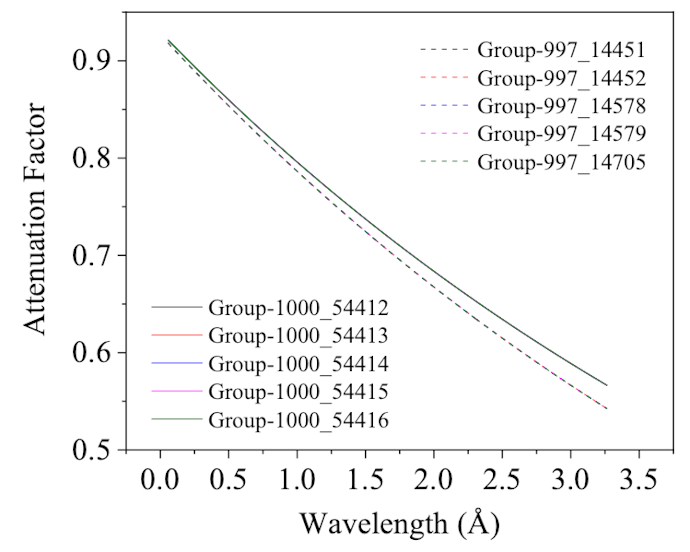
As shown in the graph above, using the KMEANS clustering algorithm, we successfully identified 1,000 groups for NOMAD detectors and two of them were picked up to demonstrate the idea. It can be clearly observed that in between different groups, the absorption spectra as the function of wavelength is distinctive, whereas for spectra within a certain group, the distinction in the absorption spectra can be ignored. This justifies our designed algorithm to only select one representative detector for the absorption calculation for each of the groups identified through the clustering algorithm. Through a test performed using a typical data set (in which ~50 Gb data is involved), with proper caching of the intermediately processed files, the overall reduction time could be reduced to ~2 minutes, in contrast to ~20 minutes with the old routine based on a pixel-by-pixel level of absorption calculation.